Quickstart

Installation

PEPFlow supports version 3.10 or newer. To install directly, use:

!pip install pepflow --quiet

Getting started

After installation, let’s run our first example with PEPFlow. We begin by importing the required libraries and creating a PEP context, which serves as the container for the problem instance and manages all elements of the PEP framework.

import pepflow as pf
import matplotlib.pyplot as plt
import numpy as np

ctx = pf.PEPContext("gd")
pf.set_current_context(ctx)

Next, we set up the performance estimation problem (PEP). We declare the four ingredients of algorithm analysis:

• function class: \(L\)-smooth convex functions;

• algorithm of interest: gradient descent method;

• initial condition: initial point and optimum are not too far away \(\|x_0 - x_\star\|^2 \leq 1\);

• performance metric: objective gap \(f(x_k) - f(x_\star)\).

pep_builder = pf.PEPBuilder(ctx)
f = pf.SmoothConvexFunction(is_basis=True, tags=["f"], L=1)
x_star = f.set_stationary_point("x_star")
x = pf.Vector(is_basis=True, tags=["x_0"])  # Initial point
pep_builder.add_initial_constraint(((x - x_star) ** 2).le(1, name="initial_condition"))

# Define the gradient descent method
N = 8
for i in range(N):
    x = x - f.grad(x)
    x.add_tag(f"x_{i + 1}")

opt_values = []
for k in range(1, N):
    x_k = ctx[f"x_{k}"]
    pep_builder.set_performance_metric(f(x_k) - f(x_star))
    result = pep_builder.solve()
    opt_values.append(result.opt_value)

plt.scatter(range(1, N), opt_values, color="blue", marker="o");

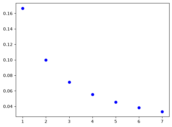
Each scatter point gives an upper bound on the objective gap that holds for all \(L\)-smooth convex functions after the corresponding number of gradient descent steps; such convergence guarantees are known as worst-case bounds.

We compare the numerical values with the analytical rate:

\[ f(x_k) - f(x_\star) \leq \frac{L}{4k+2} \|x_0 - x_\star\|_2^2. \]

iters = np.arange(1, N)
cont_iters = np.arange(1, N, 0.01)
plt.plot(
    cont_iters,
    1 / (4 * cont_iters + 2),
    "r-",
    label="Analytical bound $\\frac{1}{4k+2}$",
)
plt.scatter(iters, opt_values, color="blue", marker="o", label="Numerical values")
plt.legend();

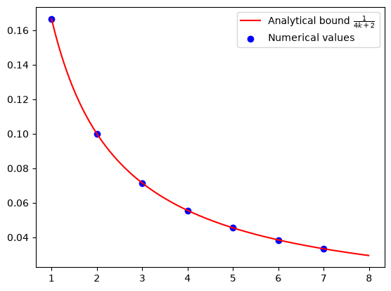
The numerical results from PEPFlow match the theoretical convergence rate.

Congratulations

You’ve just run your first PEPFlow example!

To explore PEPFlow further, users are encouraged to begin with the Tutorial, which introduces the PEP theory and showcases how PEPFlow helps derive analytical proofs corresponding to the numerical results shown above.