Accelerated Proximal Point Method (APPM) Example#
This code tests the Accelerated Proximal Point Method which is the exact optimal method that reduces the fixed-point residual \(||x - J_{\alpha A}x||\) with respect to the initial distance to the solution for a maximal monotone operator A. It was introduced in “Accelerated proximal point method for maximally monotone operators” by Donghwan Kim (2021). This method is equivalent to what later came to be known as the Optimized Halpern Method, which was studied in “On the Convergence Rate of the Halpern Iteration” by Felix Lieder (2021). The details of the equivalence can be found in Exercise 12.10 of Large-Scale Convex Optimization: Algorithms & Analyses via Monotone Operators by Ernest K. Ryu and Wotao Yin (2022).
Import the required libraries#
import pepflow as pf
import numpy as np
import sympy as sp
import matplotlib.pyplot as plt
from IPython.display import display
Define the operators#
A = pf.MonotoneOperator(is_basis=True, tags=["A"])
Write a function to return the PEPContext associated with APPM#
def make_ctx_appm(
    ctx_name: str, N: int | sp.Integer, stepsize: pf.Parameter
) -> pf.PEPContext:
    ctx_appm = pf.PEPContext(ctx_name).set_as_current()
    x = pf.Vector(is_basis=True, tags=["x_0"])
    y = x.add_tag("y_0")
    A.set_zero_point("x_star")
    for i in range(N):
        x = A.resolvent(y, stepsize, tag=f"x_{i + 1}")
        y = (
            sp.S(i + 1) / sp.S(i + 2) * (sp.S(2) * x - y)
            + sp.S(1) / sp.S(i + 2) * ctx_appm["x_0"]
        ).add_tag(f"y_{i + 1}")

    return ctx_appm
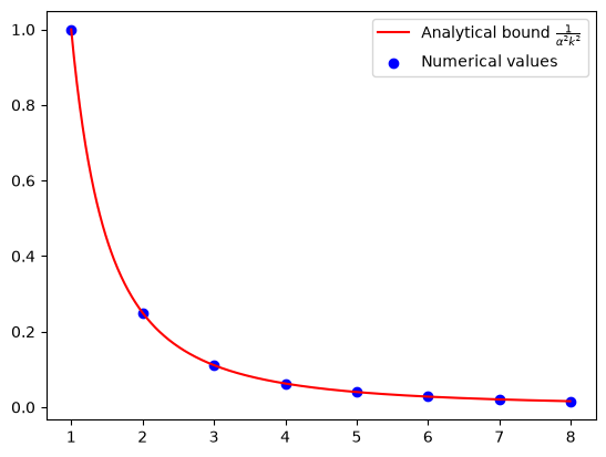
Numerical evidence of convergence of APPM#
N = 8
alpha = pf.Parameter("alpha")
R = pf.Parameter("R")
alpha_value = 1
R_value = 1

ctx_plt = make_ctx_appm(ctx_name="ctx_plt", N=N, stepsize=alpha)
pb_plt = pf.PEPBuilder(ctx_plt)
pb_plt.add_initial_constraint(
    ((ctx_plt["x_0"] - ctx_plt["x_star"]) ** 2).le(R, name="initial_condition")
)

opt_values = []
for k in range(1, N + 1):
    x_k = ctx_plt[f"x_{k}"]
    pb_plt.set_performance_metric(A(x_k) ** 2)
    result = pb_plt.solve(resolve_parameters={"alpha": alpha_value, "R": R_value})
    opt_values.append(result.opt_value)

iters = np.arange(1, N + 1)
cont_iters = np.arange(1, N, 0.01)
plt.plot(
    cont_iters,
    1 / (alpha_value**2 * cont_iters**2),
    "r-",
    label="Analytical bound $\\frac{1}{\\alpha^2 k^2}$",
)
plt.scatter(iters, opt_values, color="blue", marker="o", label="Numerical values")
plt.legend()
<matplotlib.legend.Legend at 0x7fd089cbf550>
Verification of convergence of APPM#
N = sp.S(4)
alpha_value = sp.S(1)
R_value = sp.S(1)

ctx_prf = make_ctx_appm(ctx_name="ctx_prf", N=N, stepsize=alpha)
pb_prf = pf.PEPBuilder(ctx_prf)
pb_prf.add_initial_constraint(
    ((ctx_prf["x_0"] - ctx_prf["x_star"]) ** 2).le(R, name="initial_condition")
)
pb_prf.set_performance_metric(A(ctx_prf[f"x_{N}"]) ** 2)

result = pb_prf.solve(resolve_parameters={"alpha": alpha_value, "R": R_value})
print(result.opt_value)

# Dual variables associated with the interpolations conditions of f with no relaxation
lamb_dense = result.get_scalar_constraint_dual_value_in_numpy(A)
0.06250301959936436
pf.launch_primal_interactive(
    pb_prf, ctx_prf, resolve_parameters={"alpha": alpha_value, "R": R_value}
)
Dash app running on http://127.0.0.1:8050/
It turns out for APPM no further relaxation is needed. Now we store the results.
# Dual variable associated with the initial condition
tau_sol = result.dual_var_manager.dual_value("initial_condition")
# Dual variable associated with the interpolations conditions of A
lamb_sol = result.get_scalar_constraint_dual_value_in_numpy(A)
# Dual variable associated with the Gram matrix G
S_sol = result.get_gram_dual_matrix()
Verify closed form expression of \(\lambda\)#
def tag_to_index(tag, N=N):
    """This is a function that takes in a tag of an iterate and returns its index.
    We index "x_star" as "N+1 where N is the last iterate.
    """
    # Split the string on "_" and get the index
    if (idx := tag.split("_")[1]).isdigit():
        return int(idx)
    elif idx == "star":
        return N + 1
Print the values of \(\lambda\) obtained from the solver
lamb_sol.pprint()
Consider proper candidate of closed form expression of \(\lambda\)
def lamb(tag_i, tag_j, N=N):
    i = tag_to_index(tag_i)
    j = tag_to_index(tag_j)
    if j - 1 == i:
        if j == N + 1:
            return sp.S(2) / N  ## Between N and optimal
        else:
            return sp.S(2) * (sp.S(j) - sp.S(1)) * sp.S(j) / N**2  ## Consecutive
    return 0


lamb_cand = pf.pprint_labeled_matrix(
    lamb, lamb_sol.row_names, lamb_sol.col_names, return_matrix=True
)
Check whether our candidate of \(\lambda\) matches with solution
print(
    "Did we guess the right closed form of lambda?",
    np.allclose(lamb_cand, lamb_sol.matrix, atol=1e-3),
)
Did we guess the right closed form of lambda? True
Closed form expression of \(S\)#
S_sol.pprint()
ctx_prf.basis_vectors()
[y_0, x_star, A(x_1), A(x_2), A(x_3), A(x_4)]
x_0 = ctx_prf["x_0"]
x_N = ctx_prf[f"x_{N}"]
x_star = ctx_prf["x_star"]

S_guess = (A(x_N) - 1 / (alpha * N) * (x_0 - x_star)) ** 2

pm = pf.ExpressionManager(ctx_prf, resolve_parameters={"alpha": sp.S(1)})
S_guess_eval = pm.eval_scalar(S_guess).matrix
pf.pprint_labeled_matrix(S_guess_eval, S_sol.row_names, S_sol.col_names)
print(
    "Did we guess the right closed form of S?",
    np.allclose(S_guess_eval, S_sol.matrix, atol=1e-3),
)
Did we guess the right closed form of S? True
Verify symbolic calculation for fixed \(N\)#
interpolation_scalar_sum = 0
for i in range(N + 2):
    for j in range(N + 2):
        xi = "x_star" if i == N + 1 else f"x_{i}"
        xj = "x_star" if j == N + 1 else f"x_{j}"
        if lamb(xi, xj) != 0:
            interpolation_scalar_sum += lamb(xi, xj) / alpha * A.interp_ineq(xi, xj)

interpolation_scalar_sum
RHS = interpolation_scalar_sum - S_guess
display(RHS)
LHS = A(x_N) ** 2 - 1 / (alpha**2 * N**2) * (x_0 - x_star) ** 2
display(LHS)
difference = LHS - RHS
display(difference)
pf.pprint_str(
    difference.repr_by_basis(
        ctx_prf, sympy_mode=True, resolve_parameters={"alpha": sp.S("alpha")}
    )
)