Dual Optimal Halpern Method (Dual-OHM) Example#

This code tests the Dual Optimal Halpern Method which is another exact optimal method that reduces the fixed-point residual \(||x - Tx||\) with respect to the initial distance to the solution for a nonexpansive operator T. It was introduced in “Optimal acceleration for minimax and fixed-point problems is not unique” by TaeHo Yoon, Jaeyeon Kim, Jaewook J. Suh and Ernest K. Ryu (2024). With the one-to-one correspondence \(T = 2J_{A} - I\), the analysis for a nonexpansive T can be written solely in terms of a maximally monotone operator \(A\).

Import the required libraries#

import pepflow as pf
import numpy as np
import sympy as sp
import matplotlib.pyplot as plt
from IPython.display import display

Define the operators#

A = pf.MonotoneOperator(is_basis=True, tags=["A"])

Write a function to return the PEPContext for Dual-OHM with \(T=2J_A - I\)#

def make_ctx_dual_ohm(ctx_name: str, N: int | sp.Integer) -> pf.PEPContext:
    ctx_dual_ohm = pf.PEPContext(ctx_name).set_as_current()
    y = pf.Vector(is_basis=True, tags=["y_0"])
    A.set_zero_point("y_star")
    Ty_prev = y
    for i in range(N):
        x = A.resolvent(y, sp.S(1), tag=f"x_{i + 1}")
        Ty = 2 * x - y
        y = (
            y + (sp.S(N) - sp.S(i) - sp.S(1)) / (sp.S(N) - sp.S(i)) * (Ty - Ty_prev)
        ).add_tag(f"y_{i + 1}")
        Ty_prev = Ty

    return ctx_dual_ohm

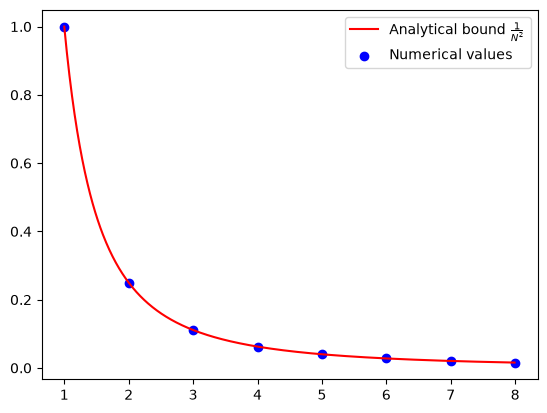
Numerical evidence on the convergence guarantee for Dual-OHM#

N_max = 8
R = pf.Parameter("R")
R_value = 1

opt_values = []
for N in range(1, N_max + 1):
    ctx_N = make_ctx_dual_ohm(ctx_name=f"ctx_{N}", N=N)
    pb_plt = pf.PEPBuilder(ctx_N)
    pb_plt.add_initial_constraint(
        ((ctx_N["y_0"] - ctx_N["y_star"]) ** 2).le(R, name="initial_condition")
    )
    x_N = ctx_N[f"x_{N}"]
    pb_plt.set_performance_metric(A(x_N) ** 2)
    result = pb_plt.solve(resolve_parameters={"R": R_value})
    opt_values.append(result.opt_value)

iters = np.arange(1, N_max + 1)
cont_iters = np.arange(1, N, 0.01)
plt.plot(
    cont_iters,
    1 / (cont_iters**2),
    "r-",
    label="Analytical bound $\\frac{1}{N^2}$",
)
plt.scatter(iters, opt_values, color="blue", marker="o", label="Numerical values")
plt.legend()

<matplotlib.legend.Legend at 0x7f9472d262d0>

../_images/cfeeb64fced0d4f5bf33b18a968051f393864ee19d7c5e01c4d64fc145062853.png

Verification of convergence of APPM#

N = sp.S(4)
R_value = sp.S(1)

ctx_prf = make_ctx_dual_ohm(ctx_name="ctx_prf", N=N)
pb_prf = pf.PEPBuilder(ctx_prf)
pb_prf.add_initial_constraint(
    ((ctx_prf["y_0"] - ctx_prf["y_star"]) ** 2).le(R, name="initial_condition")
)
pb_prf.set_performance_metric(A(ctx_prf[f"x_{N}"]) ** 2)

result = pb_prf.solve(resolve_parameters={"R": R_value})
print(result.opt_value)

# Dual variables associated with the interpolations conditions of f with no relaxation
lamb_dense = result.get_scalar_constraint_dual_value_in_numpy(A)

0.06249979133182023

pf.launch_primal_interactive(pb_prf, ctx_prf, resolve_parameters={"R": R_value})

Dash app running on http://127.0.0.1:8050/

It turns out that Dual-OHM would need no further relaxation. Now we store the results.

# Dual variable associated with the initial condition
tau_sol = result.dual_var_manager.dual_value("initial_condition")
# Dual variable associated with the interpolations conditions of A
lamb_sol = result.get_scalar_constraint_dual_value_in_numpy(A)
# Dual variable associated with the Gram matrix G
S_sol = result.get_gram_dual_matrix()

Verify closed form expression of \(\lambda\)#

def tag_to_index(tag, N=N):
    """This is a function that takes in a tag of an iterate and returns its index.
    We index "x_star" as "N+1 where N is the last iterate.
    """
    # Split the string on "_" and get the index
    if (idx := tag.split("_")[1]).isdigit():
        return int(idx)
    elif idx == "star":
        return N + 1

Print the values of \(\lambda\) obtained from the solver

lamb_sol.pprint()

\[\begin{split}\displaystyle \displaystyle \begin{array}{c|cccc} & x_2 & x_3 & x_4 & y_\star \\ \hline x_1 & 0.0 & 0.0 & 0.167 & 0.0 \\x_2 & 0.0 & 0.0 & 0.333 & 0.0 \\x_3 & 0.0 & 0.0 & 1.0 & 0.0 \\x_4 & 0.0 & 0.0 & 0.0 & 0.5 \\ \end{array} \end{split}\]

Consider proper candidate of closed form expression of \(\lambda\)

def lamb(tag_i, tag_j, N=N):
    i = tag_to_index(tag_i)
    j = tag_to_index(tag_j)
    if j == N and i < N:
        return sp.S(2) / ((N - i) * (N - i + 1))
    if j == N + 1 and i == N:
        return sp.S(2) / N  ## Between N and optimal
    return 0


lamb_cand = pf.pprint_labeled_matrix(
    lamb, lamb_sol.row_names, lamb_sol.col_names, return_matrix=True
)

Check whether our candidate of \(\lambda\) matches with solution

print(
    "Did we guess the right closed form of lambda?",
    np.allclose(lamb_cand, lamb_sol.matrix, atol=1e-3),
)

Did we guess the right closed form of lambda? True

Closed form expression of \(S\)#

S_sol.pprint()

\[\begin{split}\displaystyle \displaystyle \begin{array}{c|cccccc} & y_0 & y_\star & A(x_1) & A(x_2) & A(x_3) & A(x_4) \\ \hline y_0 & 0.062 & -0.062 & 0.0 & -0.0 & 0.0 & -0.25 \\y_\star & -0.062 & 0.062 & -0.0 & 0.0 & -0.0 & 0.25 \\A(x_1) & 0.0 & -0.0 & 0.0 & -0.0 & 0.0 & -0.0 \\A(x_2) & -0.0 & 0.0 & -0.0 & 0.0 & -0.0 & 0.0 \\A(x_3) & 0.0 & -0.0 & 0.0 & -0.0 & 0.0 & -0.0 \\A(x_4) & -0.25 & 0.25 & -0.0 & 0.0 & -0.0 & 1.0 \\ \end{array} \end{split}\]

ctx_prf.basis_vectors()

[y_0, y_star, A(x_1), A(x_2), A(x_3), A(x_4)]

y_0 = ctx_prf["y_0"]
x_N = ctx_prf[f"x_{N}"]
y_star = ctx_prf["y_star"]

S_guess = (A(x_N) - 1 / N * (y_0 - y_star)) ** 2

pm = pf.ExpressionManager(ctx_prf, resolve_parameters={})
S_guess_eval = pm.eval_scalar(S_guess).matrix
pf.pprint_labeled_matrix(S_guess_eval, S_sol.row_names, S_sol.col_names)

\[\begin{split}\displaystyle \displaystyle \begin{array}{c|cccccc} & y_0 & y_\star & A(x_1) & A(x_2) & A(x_3) & A(x_4) \\ \hline y_0 & 0.062 & -0.062 & 0.0 & 0.0 & 0.0 & -0.25 \\y_\star & -0.062 & 0.062 & 0.0 & 0.0 & 0.0 & 0.25 \\A(x_1) & 0.0 & 0.0 & 0.0 & 0.0 & 0.0 & 0.0 \\A(x_2) & 0.0 & 0.0 & 0.0 & 0.0 & 0.0 & 0.0 \\A(x_3) & 0.0 & 0.0 & 0.0 & 0.0 & 0.0 & 0.0 \\A(x_4) & -0.25 & 0.25 & 0.0 & 0.0 & 0.0 & 1.0 \\ \end{array} \end{split}\]

print(
    "Did we guess the right closed form of S?",
    np.allclose(S_guess_eval, S_sol.matrix, atol=1e-3),
)

Did we guess the right closed form of S? True

Verify symbolic calculation for fixed \(N\)#

interpolation_scalar_sum = 0
for i in np.arange(1, N + 2):
    for j in np.arange(1, N + 2):
        xi = "y_star" if i == N + 1 else f"x_{i}"
        xj = "y_star" if j == N + 1 else f"x_{j}"
        if lamb(xi, xj) != 0:
            interpolation_scalar_sum += lamb(xi, xj) * A.interp_ineq(xi, xj)

interpolation_scalar_sum

\[\displaystyle 0+1/6*-(x_1-(x_4))*(A(x_1)-A(x_4))+1/3*-(x_2-(x_4))*(A(x_2)-A(x_4))+1*-(x_3-(x_4))*(A(x_3)-A(x_4))+1/2*-(x_4-y_\star)*(A(x_4)-A(y_\star))\]

RHS = interpolation_scalar_sum - S_guess
display(RHS)

\[\displaystyle 0+1/6*-(x_1-(x_4))*(A(x_1)-A(x_4))+1/3*-(x_2-(x_4))*(A(x_2)-A(x_4))+1*-(x_3-(x_4))*(A(x_3)-A(x_4))+1/2*-(x_4-y_\star)*(A(x_4)-A(y_\star))-\|A(x_4)-1/4*(y_0-y_\star)\|^2\]

LHS = A(x_N) ** 2 - 1 / (N**2) * (y_0 - y_star) ** 2
display(LHS)

\[\displaystyle \|A(x_4)\|^2-1/16*\|y_0-y_\star\|^2\]

difference = LHS - RHS
display(difference)

\[\displaystyle \|A(x_4)\|^2-1/16*\|y_0-y_\star\|^2-(0+1/6*-(x_1-(x_4))*(A(x_1)-A(x_4))+1/3*-(x_2-(x_4))*(A(x_2)-A(x_4))+1*-(x_3-(x_4))*(A(x_3)-A(x_4))+1/2*-(x_4-y_\star)*(A(x_4)-A(y_\star))-\|A(x_4)-1/4*(y_0-y_\star)\|^2)\]

pf.pprint_str(difference.repr_by_basis(ctx_prf, sympy_mode=True))

\[\displaystyle \displaystyle 0\]

\[\begin{align*} \| \tilde{\mathbb{A}}(x^N) \|^2 - \frac{\| x^0 - x^\star \|^2}{N^2} &= -\sum_{k=1}^{N-1} \frac{2}{(N-k)(N-k+1)} \langle \tilde{\mathbb{A}}(x^N) - \tilde{\mathbb{A}}(x^k), x^N - x^k \rangle \\&\quad - \frac{2}{N} \langle \tilde{\mathbb{A}}(x^{N}), x^{N} - x^\star \rangle \\&\quad - \| \tilde{\mathbb{A}}(x^N) - \frac{1}{N} ( x^0 - x^\star) \| ^2. \end{align*}\]