Verifying numerical rates of convergence #
Let’s explore the first application of PEP: numerically verifying the rate of convergence. As an illustrative example, we consider gradient descent (GD) on \(L\)-smooth convex functions. We look for the worst function \(f\) for which, after \(N\) iterations of GD, the objective gap \(f(x_N) - f(x_\star)\) is as large as possible, where \(x_\star\) denotes a minimizer of \(f\). In other words, we obtain the worst-case convergence guarantee of GD by solving the following optimization problem
We start by setting up a PEPContext object in PEPFlow. This PEPContext object keeps track of all the mathematical objects such as points and scalars involved in the analysis.
import pepflow as pf
import numpy as np
import matplotlib.pyplot as plt

ctx = pf.PEPContext("gd").set_as_current()
More on PEPContext
The above cell not only creates a new PEPContext object called ctx, but it also sets the ctx object as the current working context. This means that all newly generated Scalar and Vector objects representing mathematical objects such as scalars and vectors/points will be automatically managed by ctx.
NB: In this tutorial, purple toggle lists provide extra details about the usage of PEPFlow. They are useful for deeper exploration or research, but can be skipped on a first read.
Then, we declare the four ingredients of algorithm analysis:
function class: \(L\)-smooth convex functions;
algorithm of interest: gradient descent method;
initial condition: initial point and optimum are not too far away \(\|x_0 - x_\star\|^2 \leq R^2\);
performance metric: objective gap \(f(x_k) - f(x_\star)\).
PEPFlow allows us to describe these objects in a high-level way that mirrors the mathematical setup. We first create a PEPBuilder object which hold all the information needed to construct and solve PEPs.
pep_builder = pf.PEPBuilder(ctx)
More on PEPBuilder
A PEPBuilder object requires passing in a PEPContext object as an argument. Using the Scalar and Vector objects managed by the PEPContext object, we can define the performance metric and initial condition for the PEPBuilder object to store.
We now define an \(L\)-smooth convex function \(f\) and set a stationary point called x_star.
L = pf.Parameter("L")

# Define function class
f = pf.SmoothConvexFunction(is_basis=True, tags=["f"], L=L)
x_star = f.set_stationary_point("x_star")
More on defining Function objects
PEPFlow offers several types of functions classes such as SmoothConvexFunction and ConvexFunction. The is_basis argument takes a boolean that designates whether the created Function object is formed as a linear combination of other Function objects. The tags argument takes in a list of strings which can be used to access the Function object through the method get_func_or_oper_by_tag. The last element of the tags list will be used to display the Function object.
More on Parameter objects
The Parameter objects can be thought of as mathematical variables. As we will see later on in the tutorial, when we perform specific operations such as solving the PEP problem, we will need to supply explicit values for the Parameter object.
More on tags
Mathematical objects in PEPFlow contain a list of user-provided strings called tags. These tags are used to access the mathematical objects easily and to display the mathematical object cleanly.
Now, we declare the initial condition \(\lVert x_0 - x_\star \rVert^2 \leq R^2\).
R = pf.Parameter("R")

# Set the initial condition
x = pf.Vector(is_basis=True, tags=["x_0"])  # The first iterate
pep_builder.add_initial_constraint(
    ((x - x_star) ** 2).le(R**2, name="initial_condition")
)
More on Vector objects
A Vector object represents an element of a pre-Hilbert space and is one of the key fundamental mathematical objects that PEPFlow provides. The is_basis argument takes a boolean that designates whether the created Vector object is formed as a linear combination of other Vector objects. The tags argument takes in a list of strings which can be used to access the Vector object easily from a context that manages it. The last element of the tags list will be used to display the Vector object.
More on ScalarConstraint objects
The code ((x - x_star) ** 2).le(R**2, name="initial_condition") creates a ScalarConstraint object which represent a scalar constraint used in the PEP. A ScalarConstraint object requires 4 components:
a
Scalarobject for the left hand side of the constraint;a
Scalarobject for the right hand side of the constraint;the type of constraint, e.g., (
le,geq,eq);a user-provided name for the constraint.
Next, we define generate the GD iterates \(\{x_i\}_{i=1}^{N}\). Note that for each iterate \(x_i\) we add a tag to display it nicely and for easy access from the PEPContext object which tracks it. Furthermore, the Vector object representing \(\nabla f(x)\) can be generated by calling f.grad(x).
N = 8
alpha = 1 / L

# Define the gradient descent method
for i in range(N):
    x = x - alpha * f.grad(x)
    x.add_tag(f"x_{i + 1}")
Tags for composite Vectors and Scalars
Vector and Scalar objects formed as linear combinations of basis objects do not have any tags. The GD iterates generated by the line of code x = x - alpha * f.grad(x) are examples of composite Vector objects. It is important for the user to give these composite objects tags to access these objects easily from the PEPContext that manages them.
Finally, we set the performance metric \(f(x_k) - f(x_\star)\). Observe that the Scalar object representing \(f(x)\) can be generated by calling f(x).
# Set the performance metric
x_N = ctx[f"x_{N}"]
pep_builder.set_performance_metric(f(x_N) - f(x_star))
Accessing Vector and Scalar objects from a PEPContext
The Vector and Scalar objects managed by a PEPContext object can be easily accessed through their tags. In the prior code block, we returned the iterate \(x_N\) represented by a Vector object with the tag x_N managed by the PEPContext object ctx through the code: ctx[f"x_{N}"].
Solving the PEP numerically gives the worst-case value of the chosen performance metric.
L_value = 1
R_value = 1
result = pep_builder.solve(resolve_parameters={"L": L_value, "R": R_value})
print(f"primal PEP optimal value = {result.opt_value:.4f}")
primal PEP optimal value = 0.0294
Resolving Parameter objects
To solve the PEP problem represented by the pep_builder object, we need to resolve the Parameter objects L and R with concrete numerical values. To do this, we pass in a dictionary of the form: {name_of_parameter: concrete_value}.
In this example, the numerical result can be interpreted as: for all \(1\)-smooth convex functions \(f\), \(8\)-step GD starting at \(x_0\) with \(\|x_0 - x_\star\|^2 \leq 1\) satisfies
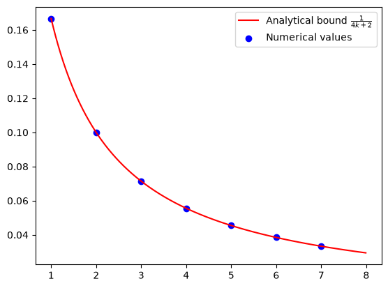
To better understand how the error decreases with the number of iterations, we repeat the process for each \(k = 1, 2, \dots, 7\). This gives us a sequence of numerical values that can be compared to the known analytical rate.
opt_values = []
for k in range(1, N):
    x_k = ctx[f"x_{k}"]
    pep_builder.set_performance_metric(f(x_k) - f(x_star))
    result = pep_builder.solve(resolve_parameters={"L": L_value, "R": R_value})
    opt_values.append(result.opt_value)

plt.scatter(range(1, N), opt_values, color="blue", marker="o");
The resulting values are visualized to show the trend of convergence. Each scatter point represents a guaranteed bound that holds for all \(L\)-smooth convex functions, while the continuous curve shows the known analytical rate for comparison (see, e.g., [1]).
After experimenting with different \(L\), \(R\), and \(N\), we tend to draw the conclusion: for all \(L\)-smooth convex functions \(f\), \(N\)-step GD with step size \(\alpha = 1/L\) satisfies
iters = np.arange(1, N)
cont_iters = np.arange(1, N, 0.01)
plt.plot(
    cont_iters,
    1 / (4 * cont_iters + 2),
    "r-",
    label="Analytical bound $\\frac{1}{4k+2}$",
)
plt.scatter(iters, opt_values, color="blue", marker="o", label="Numerical values")
plt.legend();