Deriving analytical proofs #

PEP and PEPFlow go far beyond merely numerical verification. From the dual variables (Lagrange multipliers) of Primal PEP, one can extract rigorous convergence proofs. PEPFlow bridges theory and practice by giving direct access to these dual variables and by offering an interactive environment for developing and verifying analytical proofs.

In this section, we consider a simpler running example: \(N=2\) iterations of GD. The following code block creates the PEPContext and builds the \(2\)-step GD.

import pepflow as pf
import sympy as sp
import numpy as np
import itertools
from IPython.display import display

L = pf.Parameter("L")
R = pf.Parameter("R")
N = sp.S(2)
alpha = 1 / L

ctx = pf.PEPContext("gd").set_as_current()
pep_builder = pf.PEPBuilder(ctx)

# Define function class
f = pf.SmoothConvexFunction(is_basis=True, tags=["f"], L=L)
x_star = f.set_stationary_point("x_star")

# Set the initial condition
x = pf.Vector(is_basis=True, tags=["x_0"])  # The first iterate
pep_builder.add_initial_constraint(
    ((x - x_star) ** 2).le(R**2, name="initial_condition")
)

# Define the gradient descent method
for i in range(N):
    x = x - alpha * f.grad(x)
    x.add_tag(f"x_{i + 1}")

# Set the performance metric
x_N = ctx[f"x_{N}"]
pep_builder.set_performance_metric(f(x_N) - f(x_star))

Before exploring the advanced features of PEPFlow, we first need to understand the theory behind PEP, in particular how convergence proofs can be derived through duality.

PEP theory#

From PEP to QCQP#

The PEP problem captures the spirit of a performance estimation problem: we search over all \(L\)-smooth convex functions and all GD iterates to find the scenario that maximizes the final objective gap. To make this problem tractable for computation, we need to express it entirely in terms of numerical quantities—iterates, function values, and gradient values—rather than abstract function classes. The last three sets of constraints in PEP are relatively straightforward to handle; the main difficulty lies in enforcing that \(f\) is \(L\)-smooth convex.

For \(L\)-smooth convex functions, the defining inequalities between function values, gradients, and points are well known:

\[f(x) - f(y) + \langle \nabla f(x), y-x\rangle + \tfrac{1}{L} \|\nabla f(x) - \nabla f(y)\|^2 \leq 0 \quad \text{for all} \ x, y \in \mathbf{dom} \, f.\]

This infinite collection of constraints is still intractable, as no numerical solver can handle all possible pairs \((x,y)\) in the domain of \(f\). However, the points of our interest are only those visited by the algorithm, together with the convergent optimum \(x_\star\). It is therefore natural to relax the above infinite family into a finite one:

\[f(x_j) - f(x_i) + \langle \nabla f(x_j), x_i - x_j \rangle + \tfrac{1}{L} \|\nabla f(x_i) - \nabla f(x_j)\|^2 \leq 0 \quad \text{for all} \ (x_i, x_j) \in \mathcal{K}^\star_N,\]

where the index sets \(\mathcal K^\star_N\) are defined as

(1)#\[\mathcal{I}^\star_N := \{0,1,2,\ldots,N,\star\}, \qquad \mathcal{K}^\star_N := \{(i,j) \mid i \in \mathcal{I}^\star_N, j \in \mathcal{I}^\star_N, i \neq j\}.\]

Remarkably, this relaxation turns out to be exact: the worst-case behavior of \(L\)-smooth convex functions is fully captured by these finitely many points [2]. As a result, the original problem can be formulated equivalently as a nonconvex quadratically constrained quadratic program (QCQP):

(2)#\[\begin{split}\begin{array}{ll} \text{maximize} & f_N - f_\star \\ \text{subject to} & f_j - f_i + \langle g_j, x_i - x_j \rangle + \tfrac{1}{L} \|g_i - g_j\|^2 \leq 0, \;\; (i,j) \in \mathcal{K}^\star_N \\ & x_j = x_0 - \alpha \sum_{i=0}^{j-1} g_i, \;\; j=1,2,\ldots,N \\ & \|x_0 - x_\star\|^2 \leq R^2 \\ & g_\star = 0, \end{array}\end{split}\]

where the optimization variables are \(\{(x_i, f_i, g_i)\}_{i \in \mathcal{I}^\star_N}\); recall that the index sets \(\mathcal{I}^\star_N\) and \(\mathcal{K}^\star_N\) are defined in (1). (One can view \(f_i\) as \(f(x_i)\) and \(g_i\) as \(\nabla f(x_i)\).)

Moreover, the independent or basis variables in (2) are

(3)#\[\digamma := (f_\star, f_0, f_1, \ldots, f_N) \in \mathbb R^{N+2}, \qquad \quad H := \begin{bmatrix} x_\star & x_0 & g_0 & g_1 & \cdots & g_N \end{bmatrix} \in \mathbb R^{d \times (N+3)}.\]

More specifically, entries in \(\digamma\), \(f_i\) for \(i \in \mathcal I_N^\star\), are called basis scalars and columns of \(H\) are called basis vectors. On the other hand, the variables \(\{x_1,\ldots,x_N\}\) are called non-basis variables as they are linear combinations of columns of \(H\). So, the second set of constraints in (2) describing the algorithm update rule can be removed. The non-basis variables \(x_1, x_2, \ldots, x_N\) can then be substituted directly into the first group of constraints, leaving a reduced formulation expressed entirely in terms of \(\digamma\) and \(H\).

Basis variables in PEPFlow. In PEPFlow, the elements of the decision variable \(\digamma\) are stored as Scalar objects, or EvaluatedScalar objects, if they are evaluated. Using PEPFlow we can easily see the basis scalars that a PEPContext is managing.

ctx.basis_scalars()

[f(x_star), f(x_0), f(x_1), f(x_2)]

To see the coordinates of a Scalar object, we will create an ExpressionManager object which evaluates Scalar objects and returns an EvaluatedScalar object. Let us find the EvaluatedScalar object associated with the Scalar object representing f(x_0).

x_0 = ctx["x_0"]
pm = pf.ExpressionManager(ctx, resolve_parameters={"L": sp.S(1)})
eval_sc_example = pm.eval_scalar(f(x_0))

The EvaluatedScalar object stores the information about the Scalar object’s coordinates.

pf.pprint_labeled_vector(eval_sc_example.func_coords, ctx.basis_scalars_math_exprs())

\[\begin{split}\displaystyle \displaystyle \begin{array}{cccc} f(x_\star) & f(x_0) & f(x_1) & f(x_2) \\ \hline 0.0 & 1.0 & 0.0 & 0.0 \end{array} \end{split}\]

This line of code simply means that the coordinate of \(f_0\) is \((0,1,0,0)\).

The mathematical expression and coordinate systems in PEPFlow ensure that all user inputs are represented by a mathematical expression, while all computations are carried out in coordinates automatically.

Mathematical Expressions of Basis Scalars and Basis Vectors

All Vector and Scalar objects have an underlying mathematical expression. The mathematical expressions of basis Vector and Scalar objects come from the last tag given to the object by the user. For Vector and Scalar objects formed by linear combinations of basis objects, the mathematical expression comes from the last tag given to the object by the user or, if the user did not provide any tag for the composite object, will be automatically generated from the mathematical expressions of basis objects.

The mathematical expressions of all basis scalars managed by a PEPContext ctx can be found through ctx.basis_scalars_math_exprs(). Similarly, the mathematical expressions of all basis vectors managed by a PEPContext ctx can be found through ctx.basis_vectors_math_exprs().

Retrieving \(H\) in PEPFlow

A similar argument can be made for the elements of \(H\), which are stored in PEPFlow as Vector (or EvaluatedVector) objects. The following code prints the basic vectors and the coordinate of, e.g., \(x_2\).

ctx.basis_vectors()
pm.eval_vector(ctx["x_2"]).coords

From QCQP to SDP#

It is now straightforward to transform the nonconvex QCQP (2) into a semidefinite program (SDP), which is a convex optimization problem. To do so, we introduce the Gram matrix associated with \(H\):

\[\begin{split}G := H^T H = \begin{bmatrix} \langle x_\star, x_\star \rangle & \langle x_\star, x_0 \rangle & \langle x_\star, g_0 \rangle & \langle x_\star, g_1 \rangle & \cdots & \langle x_\star, g_N \rangle \\ \langle x_0, x_\star \rangle & \ddots & & & & \vdots \\ \langle g_0, x_\star \rangle & & \ddots & & & \vdots \\ \vdots & & & & & \vdots \\ \langle g_N, x_\star \rangle & \cdots & \cdots & \cdots & \cdots & \langle g_N, g_N \rangle \end{bmatrix} \in \mathbb S^{N+3}.\end{split}\]

With this definition, every term in (2) becomes linear in \(\digamma\) and \(G\). For instance, the objective depends linearly on \(\digamma\), and inner-product terms such as \(\langle g_j, x_i \rangle\) can be expressed as \(\langle G, E \rangle\) for some coefficient matrix \(E\). Under mild conditions (e.g., \(d \geq N+3\) [1]), the QCQP (2) can be equivalently reformulated as the so-called Primal PEP:

(4)#\[\begin{split}\begin{array}{lll} \text{minimize} & \langle \digamma, c^{\text{PM}} \rangle + \langle G, C^{\text{PM}} \rangle \\ \text{subject to} & \langle \digamma, c^{\text{FC}}_{ij} \rangle + \langle G, C^{\text{FC}}_{ij} \rangle \leq 0, \;\; (i,j) \in \mathcal{K}^\star_N \\ & \langle \digamma, c^{\text{IC}} \rangle + \langle G, C^{\text{IC}} \rangle - R^2 \leq 0 \\ & G \succeq 0 \end{array}\end{split}\]

with variables \(\digamma \in \mathbb{R}^{N+2}\) and \(G \in \mathbb{S}^{N+3}\). The notation \(G \succeq 0\) means that \(G\) is symmetric positive semidefinite. Here, \((c^\text{PM}, C^\text{PM})\) correspond to the performance metric, \(\{(c^\text{FC}_{ij}, C^\text{FC}_{ij})\}\) to the function class, and \((c^\text{IC}, C^\text{IC})\) to the initial condition. We omit the explicit expressions, because PEPFlow constructs them automatically and makes them easily accessible. For example, to obtain the coefficient matrix \(E\) satisfying \(\langle G, E\rangle = \langle g_1, x_0 \rangle\):

x_1 = ctx["x_1"]
g_1 = f.grad(x_1)
pm.eval_scalar(g_1 * x_0).inner_prod_coords

array([[0. , 0. , 0. , 0. , 0. ],
       [0. , 0. , 0. , 0.5, 0. ],
       [0. , 0. , 0. , 0. , 0. ],
       [0. , 0.5, 0. , 0. , 0. ],
       [0. , 0. , 0. , 0. , 0. ]])

We are now ready to show how convergence proofs arise from duality theory. Let \(\lambda_{ij} \in \mathbb{R}\) denote the Lagrange multipliers associated with the functional constraints, \(\tau \in \mathbb{R}\) with the initial condition, and \(S \in \mathbb{S}^{N+3}\) with the PSD constraint in (4). Then the corresponding Lagrangian is

\[\begin{split}\begin{align} &\mathcal{L} (\digamma, G; \{\lambda_{ij}\}_{(i,j) \in \mathcal{K}^\star_N}, \tau, S) \\ \overset{(\blacktriangle)}{=} &\ \langle \digamma, c^\text{PM} \rangle + \langle G, C^\text{PM} \rangle - \sum_{(i,j) \in \mathcal{K}^\star_N} \lambda_{ij} (\langle \digamma, c^\text{FC}_{ij} \rangle + \langle G, C^\text{FC}_{ij} \rangle) - \tau (\langle \digamma, c^\text{IC} \rangle + \langle G, C^\text{IC} \rangle - R^2) + \langle G, S \rangle \\ \overset{(\blacktriangledown)}{=} &\ \tau R^2 + \Big\langle \digamma, c^\text{PM} - \tau c^\text{IC} - \sum_{(i,j) \in \mathcal{K}^\star_N} \lambda_{ij} c^\text{FC}_{ij} \Big\rangle + \Big\langle G, C^\text{PM} - \tau C^\text{IC} - \sum_{(i,j) \in \mathcal{K}^\star_N} \lambda_{ij} C^\text{FC}_{ij} + S \Big\rangle. \end{align}\end{split}\]

Hence, the dual of (4) is

(5)#\[\begin{split}\begin{array}{ll} \text{minimize} & \tau R^2 \\ \text{subject to} & c^\text{PM} - \tau c^\text{IC} - \sum\limits_{(i,j) \in \mathcal{K}^\star_N} \lambda_{ij} c^\text{FC}_{ij} = 0 \\ & C^\text{PM} - \tau C^\text{IC} - \sum\limits_{(i,j) \in \mathcal{K}^\star_N} \lambda_{ij} C^\text{FC}_{ij} + S = 0 \\ & \lambda_{ij} \geq 0, \;\; (i,j) \in \mathcal{K}^\star_N \\ & S \succeq 0 \end{array}\end{split}\]

with variables \(\{\lambda_{ij}\}_{(i,j) \subset \mathcal{K}^\star_N} \in \mathbb{R}\), \(\tau \in \mathbb{R}\), and \(S \in \mathbb{S}^{N+3}\).

Given any primal feasible \((\digamma, G)\) and dual feasible \((\lambda, \tau, S)\), the two inner-product terms on the right-hand side of (\(\blacktriangledown\)) are both zero and then \(\mathcal{L} = \tau R^2\). Substituting \(\mathcal{L} = \tau R^2\) back to (\(\blacktriangle\)) and reorganizing gives the identity

\[\begin{split}\begin{align} \underbrace{\langle \digamma, c^\text{PM} \rangle + \langle G, C^\text{PM} \rangle}_{\text{performance metric}} - \tau \underbrace{\big(\langle \digamma, c^\text{IC} \rangle + \langle G, C^\text{IC} \rangle \big)}_{\text{initial condition}} &\overset{(\blacksquare)}{=} \ \sum_{(i,j) \in \mathcal{K}^\star_N} \lambda_{ij} \underbrace{\big( \langle \digamma, c^\text{FC}_{ij} \rangle + \langle G, C^\text{FC}_{ij} \rangle \big)}_{\text{functional constraints}} - \underbrace{\langle G, S \rangle}_{\text{sum of squares}} \\ &\leq 0. \end{align} \end{split}\]

The inequality follows directly from primal and dual feasibility. The last inner product \(\langle G, S \rangle\) can be decomposed as sums of squares because \(G = H^TH\) is a Gram matrix—we will revisit this point later. (The derivation of (\(\blacksquare\)) is adapted from [3], with minor modifications.)

For our GD example, one can check that the equality (\(\blacksquare\)) is exactly

(6)#\[f_N - f_\star - {\tau} \| x_0 - x_\star \|^2_2 = \sum_{(i,j) \in {\mathcal K}^\star_N} {\lambda}_{ij} \Big(f_j - f_i + \langle g_j, x_i - x_j \rangle + \tfrac{1}{2L} \| g_i - g_j \|^2_2 \Big) - \langle G, S \rangle \leq 0.\]

The inequality shows that the performance metric is upper bounded by a constant multiple of the initial distance, exactly the convergence guarantee we aim to establish. In short,

a convergence guarantee is obtained via a weighted sum of all functional constraints plus a sum-of-squares term.

Hence, proving convergence reduces to verifying the equality (\(\blacksquare\)), a process known as the PEP-style proof. A PEP-style proof consists of two steps:

Step 1 dual weight identification: derive a symbolic expression for the dual variables \(\lambda_{ij}\), \((i,j) \in \mathcal{K}^\star_N\).
Step 2 Sum-of-squares (SOS) verification: confirm \(S\) is PSD, or equivalently, decompose \(\langle G, S \rangle\) into a sum of squares.

Remarkably, the equality (\(\blacksquare\)) holds for any primal feasible \((\digamma, G)\) and dual feasible \((\lambda, \tau, S)\). The tightest bound corresponds to the minimal value of \(\tau\) (or equivalently, \(\tau R^2\)), which is precisely the dual objective. Thus, a pair of primal and dual optimal points yields the tight convergence rate.

Step 1 dual weight identification#

Visualizing dual variables#

In PEPFlow, we can visualize the dual solution \(\lambda\) as follows.

result = pep_builder.solve(resolve_parameters={"L": sp.S(1), "R": sp.S(1)})
lamb_dense = result.get_scalar_constraint_dual_value_in_numpy(f)
lamb_dense.pprint()

\[\begin{split}\displaystyle \displaystyle \begin{array}{c|cccc} & x_0 & x_1 & x_2 & x_\star \\ \hline x_0 & 0.0 & 0.106 & 0.169 & 0.0 \\x_1 & 0.029 & 0.0 & 0.493 & 0.0 \\x_2 & 0.006 & 0.072 & 0.0 & 0.0 \\x_\star & 0.24 & 0.345 & 0.415 & 0.0 \\ \end{array} \end{split}\]

Return type of result.get_scalar_constraint_dual_value_in_numpy(f)

The code line result.get_scalar_constraint_dual_value_in_numpy(f) returns a MatrixWithNames object with the three member variables:

matrix: A np.ndarray containing the matrix of the dual values associated with the interpolation constraints of f;
row_names: A list of strings containing the math expressions of the points visited by f;
col_names: A list of strings containing the math expressions of the points visited by f.

The default solver in CVXPY often produces a dense \(\lambda\) matrix. The number of dual variables \(\lambda_{ij}\) grows quadratically with the number of iterations \(N\), making it impractical to infer a symbolic expression for \(\lambda\) when \(N\) is large.

However, the dual solution is not necessarily unique, and among all possible solutions, it is often desirable for \(\lambda\) to be sparse. Recall from (\(\blacksquare\)) that each \(\lambda_{ij}\) the weight assigned to the corresponding functional constraint associated with the pair \((x_i, x_j)\). When \(\lambda_{ij}=0\), the corresponding functional constraint is inactive: it does not contribute to the final convergence bound and can therefore be removed it from Primal PEP, yielding a relaxation.

In practice, a sparse \(\lambda\) is often associated with elegant analytical proofs, which rely on just a few key inequalities rather than lengthy algebraic combinations.

Exploring relaxations of Primal PEP#

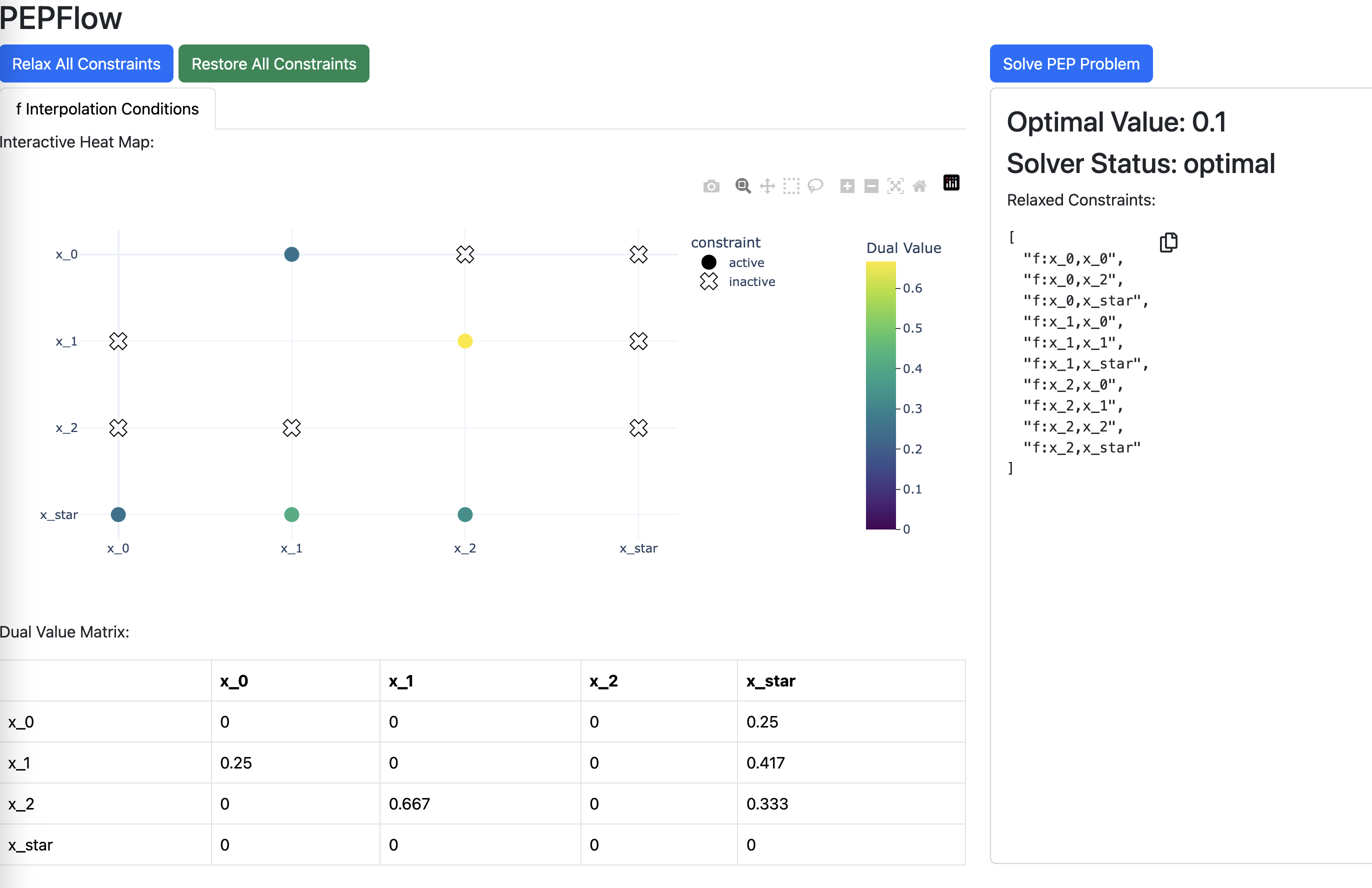
In PEPFlow, sparse \(\lambda\) can be explored in an interactive manner. In the following dashboard, users can click entries in the left matrix to set the corresponding \(\lambda_{ij}\) to zero and observe the resulting changes in real time.

# pf.launch_primal_interactive(pep_builder, ctx, resolve_parameters={"L": sp.S(1), "R": sp.S(1)})

This above line of code launches an interactive visualization of the \(\lambda\) matrix in a separate window. (A static image is shown here instead to ensure the website’s availability.)

dashboard-1

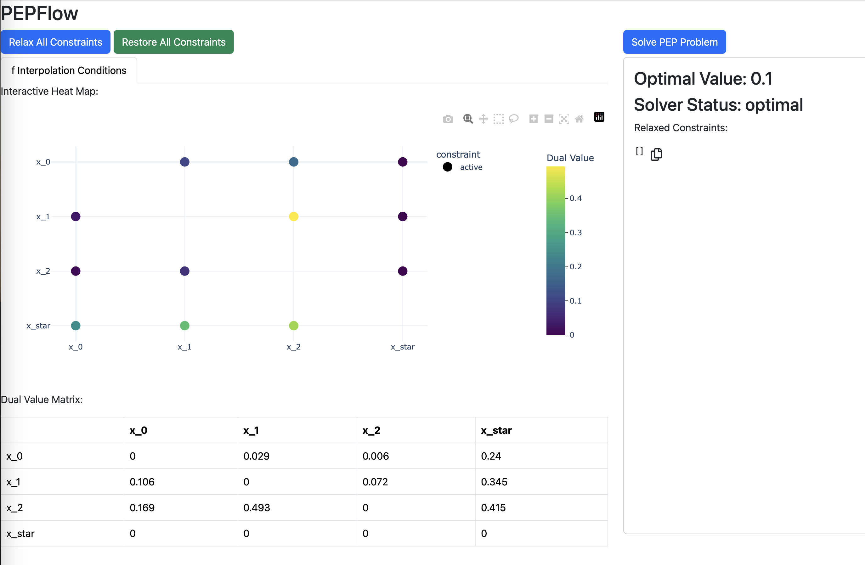
Through a few rounds of trial and error, one can identify the following sparsity pattern for \(\lambda\).

dashboard-1

With the sparsity pattern explored on the dashboard, we can solve the relaxed Primal PEP and obtain the numerical primal and dual solutions. We first write a helper function that takes in the tag of an iterate and returns the index. For example, given x_2 it will return the index 2.

def tag_to_index(tag, N=N):
    """
    This is a function that takes in a tag of an iterate and returns its index.
    We index "x_star" as "x_{N+1} where N is the last iterate.
    """

    # Split the string on "_" and get the index
    if (idx := tag.split("_")[1]).isdigit():
        return int(idx)
    elif idx == "star":
        return N + 1

The name of the interpolation constraints for the \(L\)-smooth convex function f is automatically generated by PEPFlow and are of the form f:x_i,x_j. Based on the sparsity pattern explored on the dashboard, we can remove all the constraints except those of the form f:x_{i},x_{i+1} and f:x_{i},x_{star}.

relaxed_constraints = []

for tag_i in lamb_dense.row_names:
    i = tag_to_index(tag_i)
    if i == N + 1:
        continue
    for tag_j in lamb_dense.col_names:
        j = tag_to_index(tag_j)
        if i < N and i + 1 == j:
            continue
        relaxed_constraints.append(f"f:{tag_i},{tag_j}")

pep_builder.set_relaxed_constraints(relaxed_constraints)

We now resolve the relaxed Primal PEP and store the information from the results.

result = pep_builder.solve(resolve_parameters={"L": sp.S(1), "R": sp.S(1)})

# Dual variable associated with the initial condition
tau_sol = result.dual_var_manager.dual_value("initial_condition")

# Dual variable associated with the interpolations conditions of f
lamb_sol = result.get_scalar_constraint_dual_value_in_numpy(f)

# Dual variable associated with the Gram matrix G
S_sol = result.get_gram_dual_matrix()

Return type of result.get_gram_dual_matrix()

The code line get_gram_dual_matrix() returns a MatrixWithNames object with the three member variables:

matrix: A np.ndarray containing the matrix dual variable associated with the gram matrix \(G\);
row_names: A list of strings containing the math expressions of the basis points;
col_names: A list of strings containing the math expressions of the basis points.

Find and verify symbolic expression of \(\lambda\)#

From the numerical values, we tend to consider the following candidates for the closed form expression of \(\lambda\):

\[\begin{split}\lambda_{i-1,i} = \frac{i}{2N+1-i}, \;\; i=1,\ldots,N, \qquad \quad \lambda_{\star, i} = \begin{cases} \lambda_{0,1} & i=0 \\ \lambda_{i,i+1} - \lambda_{i-1,i} \quad & i=1,\ldots,N-1 \\ 1 - \lambda_{i-1,i} & i=N, \end{cases}\end{split}\]

and other \(\lambda_{ij}\)’s are zero.

This candidate for \(\lambda\) is implemented in the following code.

def lamb(tag_i, tag_j, N=N):
    i = tag_to_index(tag_i)
    j = tag_to_index(tag_j)
    if i == N + 1:  # Additional constraint 1 (between x_★)
        if j == 0:
            return lamb("x_0", "x_1")
        elif j < N:
            return lamb(f"x_{j}", f"x_{j + 1}") - lamb(f"x_{j - 1}", f"x_{j}")
        elif j == N:
            return 1 - lamb(f"x_{N - 1}", f"x_{N}")
    if i < N and i + 1 == j:  # Additional constraint 2 (consecutive)
        return j / (2 * N + 1 - j)
    return 0


lamb_cand = pf.pprint_labeled_matrix(
    lamb, lamb_sol.row_names, lamb_sol.col_names, return_matrix=True
)

\[\begin{split}\displaystyle \displaystyle \begin{array}{c|cccc} & x_0 & x_1 & x_2 & x_\star \\ \hline x_0 & 0.0 & 0.25 & 0.0 & 0.0 \\x_1 & 0.0 & 0.0 & 0.667 & 0.0 \\x_2 & 0.0 & 0.0 & 0.0 & 0.0 \\x_\star & 0.25 & 0.417 & 0.333 & 0.0 \\ \end{array} \end{split}\]

We can check numerically whether our candidate of \(\lambda\) matches with the output solution.

print(
    "Did we guess the correct symbolic expression of lambda?",
    np.allclose(lamb_cand, lamb_sol.matrix, atol=1e-4),
)

Did we guess the correct symbolic expression of lambda? True

We can also guess and verify the symbolic expression of \(\tau\).

tau_cand = L / sp.S(4 * N + 2)

print(
    "Did we guess the correct symbolic expression of tau?",
    np.allclose(pm.eval_scalar(tau_cand), tau_sol, atol=1e-4),
)

Did we guess the correct symbolic expression of tau? True

Step 2 SOS verification#

After we find and verify the symbolic expression for \(\lambda\), the remaining task is to verify the other dual variable, \(S\), is positive semidefinite. We can visualize the numerical value of \(S\):

S_sol.pprint()

\[\begin{split}\displaystyle \displaystyle \begin{array}{c|ccccc} & x_\star & x_0 & \nabla f(x_0) & \nabla f(x_1) & \nabla f(x_2) \\ \hline x_\star & 0.1 & -0.1 & 0.125 & 0.208 & 0.167 \\x_0 & -0.1 & 0.1 & -0.125 & -0.208 & -0.167 \\\nabla f(x_0) & 0.125 & -0.125 & 0.25 & 0.208 & 0.167 \\\nabla f(x_1) & 0.208 & -0.208 & 0.208 & 0.667 & 0.167 \\\nabla f(x_2) & 0.167 & -0.167 & 0.167 & 0.167 & 0.5 \\ \end{array} \end{split}\]

With the basis system, we can easily extract the entry of \(S\) corresponding to any entry of the Gram matrix \(G\).

print(S_sol.row_names)
print(S_sol.col_names)
print(S_sol("grad_f(x_1)", "x_0"))

['x_star', 'x_0', 'grad_f(x_0)', 'grad_f(x_1)', 'grad_f(x_2)']
['x_star', 'x_0', 'grad_f(x_0)', 'grad_f(x_1)', 'grad_f(x_2)']
-0.20832653576289972

The numerical values may look complicated. But we already have its symbolic expression, from dual feasibility,

(7)#\[S = - C^\text{PM} + \tau C^\text{IC} + \sum\limits_{(i,j) \in \mathcal{K}^\star_N} \lambda_{ij} C^\text{FC}_{ij}.\]

All we need to verify is that \(S\) is PSD, or equivalently, that \(\langle G, S \rangle\) is nonnegative. Many approaches exist for this task; see, e.g.,~[1]. One convenient way is to decompose \(\langle G, S \rangle\) into a sum of squares. This approach is motivated by the fact that

\[ \langle G, S \rangle = \langle H^TH, LL^T \rangle = \|HL\|_F^2 = \sum_j \Big\|\sum_i L_{ij} h_i\Big\|^2, \]

where \(h_i\) is the \(i\)th column of \(H\) and \(S = LL^T\) is the Cholesky factorization.

In our 2-step GD example, \(H = \begin{bmatrix} x_\star & x_0 & g_0 & g_1 & g_2 \end{bmatrix}\), and so

(8)#\[\begin{split}\begin{align*} \langle G, S \rangle = \|HL\|_F^2 &= \|L_{11} x_\star + L_{21} x_0 + L_{31} g_0 + L_{41} g_1 + L_{51} g_2\|^2 \\ &\phantom{=} + \|L_{22} x_0 + L_{32} g_0 + L_{42} g_1 + L_{52} g_2\|^2 \\ &\phantom{=} \;\ \vdots \\ &\phantom{=} + \|L_{55} g_2\|^2. \end{align*}\end{split}\]

On the other hand, we see from the definition of trace that

(9)#\[\begin{split}\begin{align*} \langle G, S \rangle &= \left\langle \begin{bmatrix} \langle x_\star, x_\star \rangle & \langle x_\star, x_0 \rangle & \langle x_\star, g_0 \rangle & \langle x_\star, g_1 \rangle & \langle x_\star, g_2 \rangle \\ \langle x_0, x_\star \rangle & \ast & \ast & \ast & \ast \\ \langle g_0, x_\star \rangle & \ast & \ast & \ast & \ast \\ \langle g_0, x_\star \rangle & \ast & \ast & \ast & \ast \\ \langle g_2, x_\star \rangle & \ast & \ast & \ast & \ast \end{bmatrix}, \begin{bmatrix} S_{11} & S_{21} & S_{31} & S_{41} & S_{51} \\ S_{21} & \ast & \ast & \ast & \ast \\ S_{31} & \ast & \ast & \ast & \ast \\ S_{41} & \ast & \ast & \ast & \ast \\ S_{51} & \ast & \ast & \ast & \ast \end{bmatrix} \right\rangle \\[2pt] &= \sum_{i,j} G_{ij} S_{ij} = S_{11} \|x_\star\|^2 + 2\langle x_\star, S_{21} x_0 + S_{31} g_0 + S_{41} g_1 + S_{51} g_2 \rangle + \cdots. \end{align*}\end{split}\]

A key insight is that on the right-hand side of (8), the only term that involves \(x_\star\) is \(\|L_{11} x_\star + L_{21} x_0 + L_{31} g_0 + L_{41} g_1 + L_{51} g_2\|^2\). Combining with (9), we must have

\[L_{11} = \sqrt{S_{11}}, \qquad L_{2:5,1} = \frac{1}{L_{11}} S_{2:5,1},\]

which is exactly the first iteration of the Cholesky factorization algorithm.

Moreover, the symbolic expression of the first column of \(S\) can be extracted in a straightforward manner. We examine the three terms that define \(S\) in (7) one by one:

The first term, \(C^\text{PM}\), is zero because \(G\) does not appear in the objective.
The second term, \(C^\text{IC}\), satisfies \(\langle G, C^\text{IC} \rangle = \|x_\star - x_0\|^2\); thus, the contribution \(\tau C^\text{IC}\) corresponds to \(\tau \|x_\star - x_0\|^2\).
The terms \(C^\text{FC}_{ij}\) in the last summation correspond to the inner products \(\langle x_\star, \cdot \rangle\) appearing in the functional constraints \(f_j - f_i + \langle g_j, x_i - x_j \rangle + \tfrac{1}{L} \|g_i - g_j\|^2 \leq 0\). By inspecting the sparsity pattern of \(\lambda\), we observe that \(\lambda_{\star, i}\) is nonzero for all \(i=0,1,\ldots,N\) and \(\lambda_{j,\star} = 0\) for all \(j=0,1,\ldots,N\). Consequently, the summation in \(S\) (7) correspond to the inner product between \(x_\star\) and \(\sum_{i=0}^N \lambda_{\star, i} g_i\).

To conclude, the squared term in \(\langle G, S \rangle\) that involves \(x_\star\) is

\[ \tau \Big\|x_\star - x_0 + \frac{1}{2\tau} \sum_{i=0}^N \lambda_{\star, i} g_i \Big\|^2, \]

while all remaining terms in \(\langle G, S \rangle\) are independent of \(x_\star\).

The following code constructs the squared term involving \(x_\star\) and subtracts it from \(S\).

We first collect a list of the points visited by the function f and store the optimal solution x_star.

x = ctx.tracked_point(f)
print(x)
x_star = ctx["x_star"]

[x_0, x_1, x_2, x_star]

Now we construct the squared term involving \(x_\star\) and subtracts it from \(S\).

tau_cand = L / sp.S(4 * N + 2)

grad_terms = sum(lamb(x_star.tag, x[i].tag) * f.grad(x[i]) for i in range(N + 1))
z_N = x_star - x_0 + 1 / (2 * tau_cand) * grad_terms
iter_diff_square = tau_cand * z_N**2

remainder_1 = S_sol.matrix - pm.eval_scalar(iter_diff_square).inner_prod_coords
pf.pprint_labeled_matrix(remainder_1, S_sol.row_names, S_sol.col_names)

\[\begin{split}\displaystyle \displaystyle \begin{array}{c|ccccc} & x_\star & x_0 & \nabla f(x_0) & \nabla f(x_1) & \nabla f(x_2) \\ \hline x_\star & 0.0 & -0.0 & -0.0 & -0.0 & 0.0 \\x_0 & -0.0 & 0.0 & 0.0 & 0.0 & -0.0 \\\nabla f(x_0) & -0.0 & 0.0 & 0.094 & -0.052 & -0.042 \\\nabla f(x_1) & -0.0 & 0.0 & -0.052 & 0.233 & -0.181 \\\nabla f(x_2) & 0.0 & -0.0 & -0.042 & -0.181 & 0.222 \\ \end{array} \end{split}\]

As expected, the first column and row of \(S\) vanish, since all terms involving \(x_\star\) have been absorbed into the vector \(z\) defined above. Interestingly, the second column and row, corresponding to \(x_0\), also vanish. This is not a coincidence: in the GD example, shifting the function \(f\) by a constant does not affect the worst-case performance of gradient descent. Consequently, only the relative position between \(x_0\) and \(x_\star\) matters, not their absolute locations.

We then follow the same process and eliminate the remaining basic vectors \(g_0,g_1,\ldots,g_N\).

grad_diff_square = pf.Scalar.zero()
for i in range(N + 1):
    for j in range(i + 1, N + 1):
        const_1 = (2 * N + 1) * lamb(x_star.tag, x[i].tag) - 1
        const_2 = lamb(x_star.tag, x[j].tag)
        grad_diff_square += (
            1 / (2 * L) * (const_1 * const_2 * (f.grad(x[i]) - f.grad(x[j])) ** 2)
        )

remainder_2 = remainder_1 - pm.eval_scalar(grad_diff_square).inner_prod_coords
pf.pprint_labeled_matrix(remainder_2, S_sol.row_names, S_sol.col_names)

\[\begin{split}\displaystyle \displaystyle \begin{array}{c|ccccc} & x_\star & x_0 & \nabla f(x_0) & \nabla f(x_1) & \nabla f(x_2) \\ \hline x_\star & 0.0 & -0.0 & -0.0 & -0.0 & 0.0 \\x_0 & -0.0 & 0.0 & 0.0 & 0.0 & -0.0 \\\nabla f(x_0) & -0.0 & 0.0 & -0.0 & -0.0 & 0.0 \\\nabla f(x_1) & -0.0 & 0.0 & -0.0 & -0.0 & 0.0 \\\nabla f(x_2) & 0.0 & -0.0 & 0.0 & 0.0 & -0.0 \\ \end{array} \end{split}\]

We can easily verify our decomposition of \(S\) as follows.

S_guess = iter_diff_square + grad_diff_square

print(
    "Did we guess the right closed form of S?",
    np.allclose(pm.eval_scalar(S_guess).inner_prod_coords, S_sol.matrix, atol=1e-4),
)

Did we guess the right closed form of S? True

Symbolic calculation#

We can double check the proof identity

\[ f_N - f_\star - \tau \| x_0 - x_\star \|^2_2 = \sum\limits_{(i,j) \in {\mathcal K}^\star_N} {\lambda}_{ij} \Big(f_j - f_i + \langle g_j, x_i - x_j \rangle + \tfrac{1}{2L} \| g_i - g_j \|^2_2 \Big) - \langle G, S \rangle \]

using the symbolic computation system in Sympy.

We first assemble the summation term on RHS:

\[ \sum\limits_{(i,j) \in {\mathcal K}^\star_N} {\lambda}_{ij} \Big(f_j - f_i + \langle g_j, x_i - x_j \rangle + \tfrac{1}{2L} \| g_i - g_j \|^2_2 \Big). \]

interp_scalar_sum = pf.Scalar.zero()
for x_i, x_j in itertools.product(x, x):
    if lamb(x_i.tag, x_j.tag) != 0:
        interp_scalar_sum += lamb(x_i.tag, x_j.tag) * f.interp_ineq(x_i.tag, x_j.tag)

display(interp_scalar_sum)

Then we assemble the entire RHS

\[ \sum\limits_{(i,j) \in {\mathcal K}^\star_N} {\lambda}_{ij} \Big(f_j - f_i + \langle g_j, x_i - x_j \rangle + \tfrac{1}{2L} \| g_i - g_j \|^2_2 \Big) - \langle G, S \rangle. \]

RHS = interp_scalar_sum - S_guess
display(RHS)

We assemble the LHS in the same manner.

LHS = f(x[N]) - f(x_star) - L / (4 * N + 2) * (x[0] - x_star) ** 2
display(LHS)

\[\displaystyle f(x_2)-f(x_\star)-L/10*\|x_0-x_\star\|^2\]

We display the difference using Sympy’s symbolic computation system.

diff = LHS - RHS
display(diff)

With our basis system, we can easily simplify the above expression.

pf.pprint_str(
    diff.repr_by_basis(ctx, sympy_mode=True, resolve_parameters={"L": sp.S("L")})
)

\[\displaystyle \displaystyle 0\]

We can also verify that the coordinates of the LHS and the RHS match.

RHS_func = pm.eval_scalar(RHS).func_coords
pf.pprint_labeled_vector(RHS_func, ctx.basis_scalars_math_exprs())

LHS_func = pm.eval_scalar(LHS).func_coords
pf.pprint_labeled_vector(LHS_func, ctx.basis_scalars_math_exprs())

\[\begin{split}\displaystyle \displaystyle \begin{array}{cccc} f(x_\star) & f(x_0) & f(x_1) & f(x_2) \\ \hline -1.0 & 0.0 & 0.0 & 1.0 \end{array} \end{split}\]

RHS_ip = pm.eval_scalar(RHS).inner_prod_coords
pf.pprint_labeled_matrix(RHS_ip, ctx.basis_vectors_math_exprs())

LHS_ip = pm.eval_scalar(LHS).inner_prod_coords
pf.pprint_labeled_matrix(LHS_ip, ctx.basis_vectors_math_exprs())

\[\begin{split}\displaystyle \displaystyle \begin{array}{c|ccccc} & x_\star & x_0 & \nabla f(x_0) & \nabla f(x_1) & \nabla f(x_2) \\ \hline x_\star & -0.1 & 0.1 & 0.0 & -0.0 & 0.0 \\x_0 & 0.1 & -0.1 & 0.0 & 0.0 & 0.0 \\\nabla f(x_0) & 0.0 & 0.0 & 0.0 & 0.0 & 0.0 \\\nabla f(x_1) & -0.0 & 0.0 & 0.0 & -0.0 & -0.0 \\\nabla f(x_2) & 0.0 & 0.0 & 0.0 & -0.0 & 0.0 \\ \end{array} \end{split}\]

\[\begin{split}\displaystyle \displaystyle \begin{array}{c|ccccc} & x_\star & x_0 & \nabla f(x_0) & \nabla f(x_1) & \nabla f(x_2) \\ \hline x_\star & -0.1 & 0.1 & 0.0 & 0.0 & 0.0 \\x_0 & 0.1 & -0.1 & 0.0 & 0.0 & 0.0 \\\nabla f(x_0) & 0.0 & 0.0 & 0.0 & 0.0 & 0.0 \\\nabla f(x_1) & 0.0 & 0.0 & 0.0 & 0.0 & 0.0 \\\nabla f(x_2) & 0.0 & 0.0 & 0.0 & 0.0 & 0.0 \\ \end{array} \end{split}\]

We have shown that with the guessed symbolic expression of \((\lambda, \tau, S)\), LHS of (6) is equal to RHS for \(N=2\).

You can also try other values of \(N\) to check that the \((\lambda, \tau, S)\) candidate continues to hold, before finalizing the formal proof for the general case.

This completes the entire PEP workflow.